
For better or worse, Excel has been the backbone of office data management for many companies.
Depending on your business, the amount of data to be handled sometimes can be overwhelmingly large. And because time is money, every shortcut that spares you time and increases productivity is valuable.
For example using the mouse to select or command some operations could be time-consuming. This is especially so if the data to be handled is large – finding just one trick can save some precious minutes every day. Here are some shortcuts to help you handle your spreadsheets much easier.
1. Automatic Sum
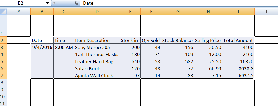
Usually if you want to find the sum of values in a spreadsheet you have to highlight the cell where the sum would go, then click auto sum and finish by hitting the ENTER key. This takes a hell lot of time only to find the sum to one column. With large data, you need a faster and friendlier way to do the sum.
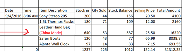
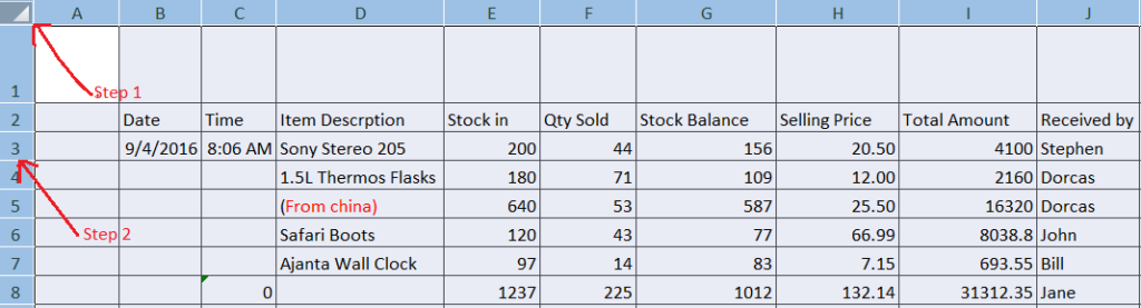
If you want to get the sum of the entire document at the bottom end of each column, just hit Ctrl + A to highlight the whole document. Then press Alt + =. This will give you the totals for all the columns with numbers in your worksheet.
Click Ctrl + A to select the document
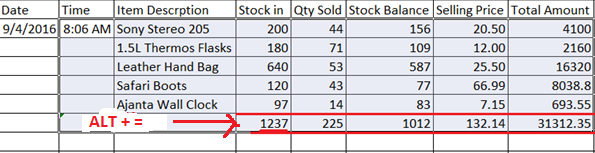
Click Alt + = to auto sum.
2. Insert Date and Time
Most of the time you need to indicate the time a transaction takes place. Date and time is important for tracking, KPIs, data for management and so on.
If you routinely type them in one by one, I have good news: you just need to use two keys and have the date and time automagically appear in a second.
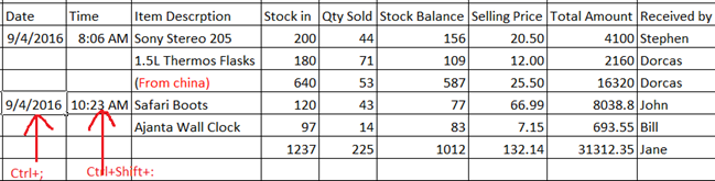
To insert the date, just press Ctrl + : (full colon).
To insert the time, press Ctrl + Shift + ; (semi-colon).
3. Highlighting a Column or a Row
When you want to work on or use the data in a whole column or a row, you don’t have to drag the mouse over the part you’re trying to select. To select a whole row of data, all you need to do is to place the cursor in one cell of the active row and the press Shift + Space.
To highlight a column, you just need to place the cursor in one of the cells in the column, then press Ctrl + Space and you’re done. A lot faster than fumbling with the mouse, isn’t it?
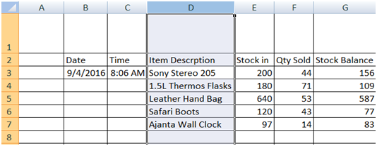
Press Ctrl + Space to highlight a column.
Press Shift + Space
4. Add a New Text Line
Even though excel is not a word processor, you surely will have to write some text in the worksheet. Maybe writing names of people or objects in one cell may require you to start new lines in the same cell.
Unlike in word, if you press the enter key excel takes you one cell lower. But if you press ALT + ENTER a new line inside the cell will be started.
5. Best Fitting Your Work In the Cells
When the data in your worksheet looks crammed, you need to give it some more space to have it look neat and presentable. When the cells are too small, your work would look messed up if it was to be printed.
You need to adjust the column width and the row height in your worksheet. Because the data in each column may not be of the same length, the columns also need different widths. A column for names needs a bigger width compared to the one for phone numbers.
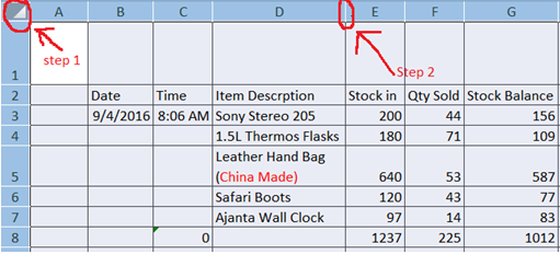
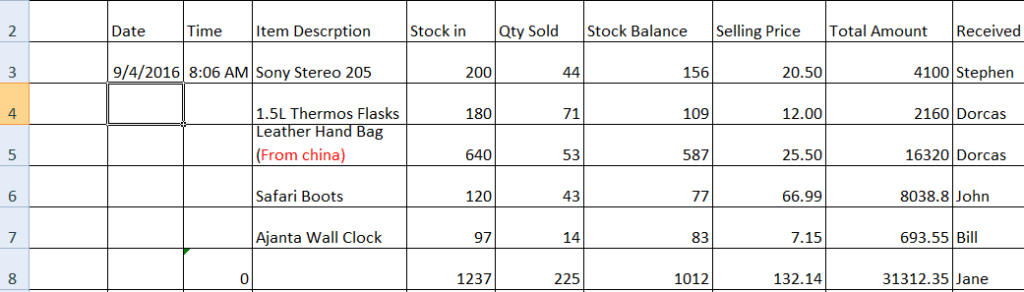
To give your work the best fit on the worksheet, click on the left-upper-corner on the outside of the A1 cell. This highlights the whole worksheet. Then you double click on any divider between two columns that have been highlighted. This sets your columns to fit well, according to the data in them without handling a column at a time.
If want to adjust your document to a uniform row height, click at the left upper corner again if your document is not selected. Place the cursor on any boundary between two cells. Click and hold on the mouse. Drag the cursor to set the desired row height. When you release the mouse, the whole document will be set to a uniform row height.
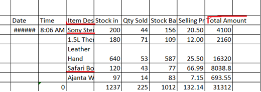
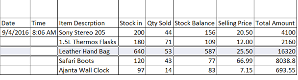
These data up here is poorly fitting
This is a Best Fit Data
To adjust row height:
6. Toggle AutoFilters
If you mostly use filters on tables and lists, sometimes you may need to remove the filters and then bring them back the next second. If you have employed several filters in the document, removing them manually can take an awfully long time.
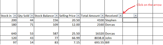
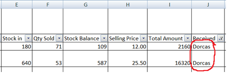
You can simply undo all the filters by using the Ctrl +Shift + L. When this is done once, it removes the filter and a repeat of the same key combination reinstates the filters. This is way much faster than working on each filter manually at a time. On pressing the keys, column arrows appear as shown below:
I hope these helped, stay tuned for more.